divraster-vignette
Flávio M. M. Mota, Neander M. Heming, and Gabriela Alves-Ferreira
2026-01-11
Source:vignettes/divraster-vignette.Rmd
divraster-vignette.Rmd- 1 Introduction
- 2 Alpha diversity
- 3 Standardized effect size (SES)
- 4 Beta diversity
- 5 Traits average
- 6 Suitability change
- 7 Area calculation
- 8 Richness difference between scenarios
- 9 Occurrence distance helper
- 10 Raster–polygon summaries
- 11 Cropping by binary footprint
1 Introduction
Macroecological studies have been increasingly utilized in the
context of climate change, necessitating the use of tools to analyze
large datasets. To examine and comprehend the intricate mechanisms that
underlie species distributions and the structure of biological
communities, a diverse array of metrics has been developed. These
metrics encompass alpha and beta diversity patterns across taxonomic
(TD), functional (FD), and phylogenetic (PD) dimensions. The package
divraster addresses a current gap in this field by offering
functions to calculate diversity metrics directly from rasters,
eliminating the need for matrix transformations. This capability is
especially valuable when dealing with extensive datasets, as matrices
often impose memory constraints.
2 Alpha calculations
Alpha diversity calculations use a tree-based approach for taxonomic (TD), functional (FD), and phylogenetic (PD) diversity. In the FD calculation, a species traits matrix is converted into a distance matrix and clustered to produce a regional dendrogram (i.e. a dendrogram with all species in the raster stack) from which the total branch length is calculated. When calculating FD for each community (i.e. raster cell), the regional dendrogram is subsetted into a local dendrogram containing only the species present on the local community, and only the branch lengths connecting them are summed to represent the functional relationships of the species locally present. Similarly, in PD, the sum of branch lengths connecting species within a community represents their shared phylogenetic relationships and cumulative evolutionary history. Alpha TD can also be visualized using a tree diagram, where each species is directly connected to the root by an edge of unit length, reflecting the number of different taxa in the community (i.e. species richness) since all taxa are at the same level.
2.1 Alpha examples
2.1.1 Alpha TD
# Loading data
# Presence-absence SpatRaster
bin1 <- terra::rast(system.file("extdata",
                                "ref_frugivor.tif",
                                package = "divraster"))
bin2 <- terra::rast(system.file("extdata",
                                "fut_frugivor.tif",
                                package = "divraster"))

# Change extension to process faster
terra::ext(bin1)
#> SpatExtent : -41.875, -38.75, -21.375, -13 (xmin, xmax, ymin, ymax)
e <- c(-40, -39, -14, -13)
bin1 <- terra::crop(bin1, e)
bin2 <- terra::crop(bin2, e)

# Species traits
traits <- read.csv(system.file("extdata",
                               "traits_frugivor.csv",
                               package = "divraster"),
                   sep = ";",
                   row.names = 1)

# Phylogenetic tree
tree <- ape::read.tree(system.file("extdata",
                                   "tree_frugivor.tre",
                                   package = "divraster"))

# Alpha TD calculation for scenario 1
divraster::spat.alpha(bin1)
#> class       : SpatRaster
#> size        : 8, 8, 1  (nrow, ncol, nlyr)
#> resolution  : 0.125, 0.125  (x, y)
#> extent      : -40, -39, -14, -13  (xmin, xmax, ymin, ymax)
#> coord. ref. : lon/lat WGS 84 (EPSG:4326)
#> source(s)   : memory
#> name        : Alpha_TD
#> min value   :        0
#> max value   :       67

# Alpha TD calculation for scenario 2
divraster::spat.alpha(bin2)
#> class       : SpatRaster
#> size        : 8, 8, 1  (nrow, ncol, nlyr)
#> resolution  : 0.125, 0.125  (x, y)
#> extent      : -40, -39, -14, -13  (xmin, xmax, ymin, ymax)
#> coord. ref. : lon/lat WGS 84 (EPSG:4326)
#> source(s)   : memory
#> name        : Alpha_TD
#> min value   :        0
#> max value   :       65
The alpha taxonomic diversity in the first scenario ranges from 0 to 67, and in the second scenario, it ranges from 0 to 65, with higher values concentrated towards the north in both cases.
2.1.2 Alpha FD
divraster::spat.alpha(bin1, traits)The alpha functional diversity for the first scenario ranges from 4.248408 to 4.378846, with higher values concentrated towards the north, indicating greater functional diversity.
2.1.3 Alpha PD
# Alpha PD calculation
divraster::spat.alpha(bin1, tree)
#> class       : SpatRaster
#> size        : 8, 8, 1  (nrow, ncol, nlyr)
#> resolution  : 0.125, 0.125  (x, y)
#> extent      : -40, -39, -14, -13  (xmin, xmax, ymin, ymax)
#> coord. ref. : lon/lat WGS 84 (EPSG:4326)
#> source(s)   : memory
#> name        : Alpha_PD
#> min value   : 1793.342
#> max value   : 1859.668
The alpha phylogenetic diversity for the first scenario ranges from 1793.342 to 1859.668, with higher values concentrated towards the north, indicating greater phylogenetic diversity.
3 Standardized effect size (SES)
SES is often used in ecological studies to measure the magnitude of
difference between observed and randomized patterns generated by null
models, expressed in standard deviation units. We calculate SES using
the SESraster package, which currently offers six community
randomization methods. The basic randomization methods include: keeping
the richness constant and randomizing the position of the species within
each raster cell (site), keeping range size constant and randomizing the
position of species presences in space (species), and randomizing by
both site and species simultaneously (both). A positive SES indicates
that the observed functional/phylogenetic diversity is higher than
expected solely based on species richness (taxonomic diversity), whereas
a negative SES indicates the opposite.
3.1.1 SES FD
# SES FD calculation
divraster::spat.rand(x = bin1,
                     tree = traits,
                     aleats = 3,
                     random = "site")
The SES indicates that the majority of the areas have values close to 0, suggesting that functional diversity does not significantly differ from the expected change. However, one community is projected to be functionally clustered (SES_FD = -25).
3.1.2 SES PD
# SES PD calculation
divraster::spat.rand(x = bin1,
                     tree = tree,
                     aleats = 3,
                     random = "site")
In contrast, the SES for phylogenetic diversity does not differ from what is expected by chance, with most communities presenting values close to 0. However, one community is projected to be phylogenetically dispersed (SES_PD = 12).
4 Beta diversity
Beta diversity captures variations in species composition between different communities. When examining a community in comparison to its neighboring ones, it is referred to as spatial beta diversity. On the other hand, when assessing changes within the same community over different time periods, it is termed temporal beta diversity. Beta diversity can further be partitioned into two components: “replacement” and “richness differences”. The former accounts for the substitution of one species with another, while the latter encompasses discrepancies in the total number of species (e.g. species gain or loss). In addition, since Btotal represents the sum of Brepl and Brich components, the proportion of Brepl/Btotal (Bratio) can be calculated, with values close to 0 indicating the predominance of Brich and values close to 1 indicating the predominance of Brepl. Moreover, the concept of beta diversity extends to functional (FD) and phylogenetic diversity (PD), using the same framework as taxonomic diversity (TD). In the context of TD, higher beta diversity represents higher dissimilarities in species composition between communities. In contrast, for FD, it indicates higher dissimilarities in functional traits, and for PD, it reflects higher dissimilarities in phylogenetic relationships of species between communities.
4.1.1 Beta spatial TD
# Beta spatial TD calculation
divraster::spat.beta(bin1)
Spatial beta diversity for TD indicates a slight change in species composition towards the south, as evidenced by the small values of Btotal (ranging from 0.002985075 to 0.045232793). The predominant component contributing to this change is the richness difference (Brich), suggesting that dissimilarities between each community (i.e. pixel) and its neighbors are primarily due to the loss or gain of species.
4.1.2 Beta spatial FD
# Beta spatial FD calculation
divraster::spat.beta(bin1, traits)
Similarly, spatial beta diversity for FD indicates a slight change in functional traits composition towards the south, as evidenced by the small values of Btotal (ranging from 0.0001674408 to 0.0235750070). The predominant component contributing to this little change is the richness difference (Brich), suggesting that dissimilarities between each community (i.e. pixel) and its neighbors are primarily due to the loss or gain of functional traits.
4.1.3 Beta spatial PD
# Beta spatial PD calculation
divraster::spat.beta(bin1, tree)
The spatial beta diversity for PD also indicates a slight change in the evolutionary history of communities towards the south, as evidenced by the small values of Btotal (ranging from 0.0008262028 to 0.0190497319). The predominant component contributing to this little change is also the richness difference (Brich), suggesting that dissimilarities between each community (i.e. pixel) and its neighbors are due to the loss or gain of evolutionary history.
4.1.4 Beta temporal TD
# Beta temporal TD calculation
divraster::temp.beta(bin1, bin2)
#> class       : SpatRaster
#> size        : 8, 8, 4  (nrow, ncol, nlyr)
#> resolution  : 0.125, 0.125  (x, y)
#> extent      : -40, -39, -14, -13  (xmin, xmax, ymin, ymax)
#> coord. ref. : lon/lat WGS 84 (EPSG:4326)
#> source(s)   : memory
#> names       :  Btotal_TD,   Brepl_TD,   Brich_TD, Bratio_TD
#> min values  : 0.02985075, 0.00000000, 0.02985075, 0.0000000
#> max values  : 0.13636364, 0.06153846, 0.13636364, 0.5714286
The temporal beta diversity for TD indicates that future communities in the north are expected to experience changes in their species composition. This is driven by the Brich component, suggesting these dissimilarities are attributed to gains or losses of species.
4.1.5 Beta temporal FD
# Beta temporal FD calculation
divraster::temp.beta(bin1, bin2, traits)
#> class       : SpatRaster
#> size        : 8, 8, 4  (nrow, ncol, nlyr)
#> resolution  : 0.125, 0.125  (x, y)
#> extent      : -40, -39, -14, -13  (xmin, xmax, ymin, ymax)
#> coord. ref. : lon/lat WGS 84 (EPSG:4326)
#> source(s)   : memory
#> names       :  Btotal_FD,   Brepl_FD,    Brich_FD, Bratio_FD
#> min values  : 0.01358064, 0.00000000, 0.007364383, 0.0000000
#> max values  : 0.07041225, 0.02160415, 0.070412255, 0.7457799
The temporal beta diversity for FD indicates a less pronounced pattern compared to TD, with smaller values of Btotal. The Brich component is also predominant, suggesting that the small dissimilarities can be attributed to gains or losses of functional traits.
4.1.6 Beta temporal PD
# Beta temporal PD calculation
divraster::temp.beta(bin1, bin2, tree)
#> class       : SpatRaster
#> size        : 8, 8, 4  (nrow, ncol, nlyr)
#> resolution  : 0.125, 0.125  (x, y)
#> extent      : -40, -39, -14, -13  (xmin, xmax, ymin, ymax)
#> coord. ref. : lon/lat WGS 84 (EPSG:4326)
#> source(s)   : memory
#> names       :  Btotal_PD,  Brepl_PD,   Brich_PD, Bratio_PD
#> min values  : 0.01202170, 0.0000000, 0.01202170, 0.0000000
#> max values  : 0.08652411, 0.0394096, 0.08652411, 0.6232362
Likewise, the temporal beta diversity for PD indicates a less pronounced pattern compared to TD, with smaller values of Btotal. The Brich component is also predominant, suggesting that the small dissimilarities can be attributed to gains or losses of evolutionary history.
5 Traits average
Calculating the average traits of species for each climate scenario enables the evaluation of species traits that contribute the most to the loss of suitable habitat. Unlike functional diversity, which combines functional traits into an index, this approach provides direct insight into spatial variations in average traits. This information can complement the data necessary for delineating conservation priority areas, as shifts in average traits—whether increasing or decreasing—indicate the potential loss of species with specific features. This is of particular significance given that functional traits are closely tied to the ecological services provided by species.
5.1 Traits average examples
# Average traits calculation
# Scenario 1
divraster::spat.trait(bin1, traits)
#> class       : SpatRaster
#> size        : 8, 8, 12  (nrow, ncol, nlyr)
#> resolution  : 0.125, 0.125  (x, y)
#> extent      : -40, -39, -14, -13  (xmin, xmax, ymin, ymax)
#> coord. ref. : lon/lat WGS 84 (EPSG:4326)
#> source(s)   : memory
#> names       : Beak.~ulmen, Beak.~Nares, Beak.Width, Beak.Depth, Tarsu~ength, Wing.Length, ...
#> min values  :    23.95758,    15.97879,   7.613636,   9.250000,    25.55224,    117.9833, ...
#> max values  :    24.36250,    16.28333,   7.804545,   9.601515,    25.89531,    120.3712, ...

# Scenario 2
divraster::spat.trait(bin2, traits)
#> class       : SpatRaster
#> size        : 8, 8, 12  (nrow, ncol, nlyr)
#> resolution  : 0.125, 0.125  (x, y)
#> extent      : -40, -39, -14, -13  (xmin, xmax, ymin, ymax)
#> coord. ref. : lon/lat WGS 84 (EPSG:4326)
#> source(s)   : memory
#> names       : Beak.~ulmen, Beak.~Nares, Beak.Width, Beak.Depth, Tarsu~ength, Wing.Length, ...
#> min values  :    23.22833,    15.01000,   7.336667,   8.918333,    25.65077,    118.2877, ...
#> max values  :    25.15000,    16.84655,   7.905172,   9.598276,    26.57241,    122.3655, ...
The average beak depth in the first scenario ranges from 9.25 to 9.6, while in the second scenario, it ranges from 8.9 to 9.6. The reduction in beak size can be attributed to the decline of species with larger beak depths.
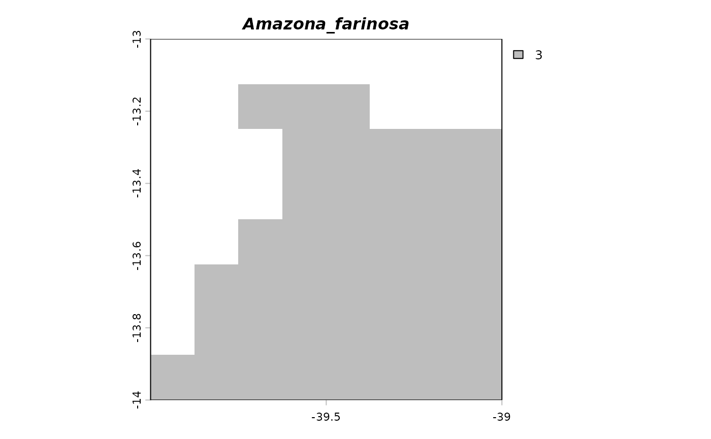
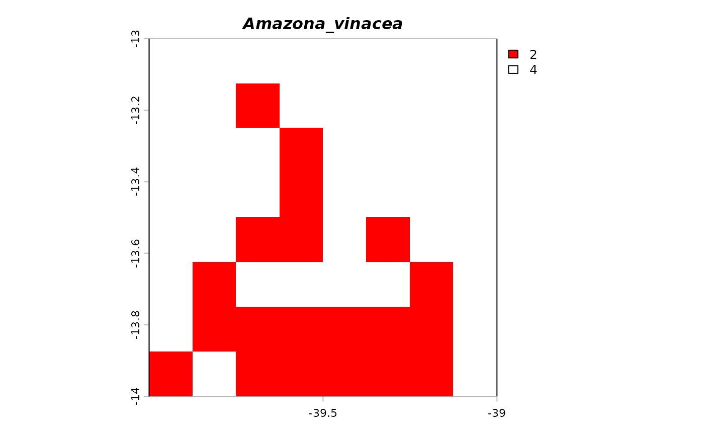
6 Suitability change
# Suitability change between climate scenarios
change <- divraster::suit.change(bin1[[1:4]], bin2[[1:4]])

# Visualization
# Initialize an empty list to store color mappings for each layer
change.col <- list()

# Loop through each layer in the 'change' raster
for(i in 1:terra::nlyr(change)){
  # Get unique values, omitting NA values, and sort them
  change.col[[i]] <- sort(na.omit(unique(terra::values(change[[i]]))))

  # Map numeric values to specific colors
  change.col[[i]][change.col[[i]] == 1] <- "blue"   # Gain
  change.col[[i]][change.col[[i]] == 2] <- "red"    # Loss
  change.col[[i]][change.col[[i]] == 3] <- "grey"   # No change
  change.col[[i]][change.col[[i]] == 4] <- "white"  # Unsuitable

  # Plot the change in suitability
  terra::plot(change[[i]], col = change.col[[i]],
              main = names(change)[i],
              cex.main = 1,
              font.main = 4)
}


 Suitability change between climate scenarios with values equals 1
representing gain, values equals 2 representing loss, values equals 3
representing no change, and values equals 4 representing unsuitable in
both scenarios.
7 Area calculation
# Climate suitable area scenario 1
divraster::area.calc(bin1[[1:4]])
#>                   Layer     Area
#> 1      Amazona_farinosa 7686.712
#> 2  Amazona_rhodocorytha 7686.712
#> 3       Amazona_vinacea 3749.616
#> 4 Arremon_semitorquatus    0.000

# Climate suitable area scenario 2
divraster::area.calc(bin2[[1:4]])
#>                   Layer     Area
#> 1      Amazona_farinosa 7686.712
#> 2  Amazona_rhodocorytha 7686.712
#> 3       Amazona_vinacea    0.000
#> 4 Arremon_semitorquatus    0.000
The climate suitable area for species such as Amazona farinosa is expected to remain the same (7,686 km), while for species such as Amazona vinacea climate suitability is expected to be eliminated (a 100% reduction).
8 Richness difference between scenarios
# Difference in species richness between climate scenarios
divraster::differ.rast(divraster::spat.alpha2(bin1),
                       divraster::spat.alpha2(bin2), perc = FALSE)
#> class       : SpatRaster
#> size        : 8, 8, 1  (nrow, ncol, nlyr)
#> resolution  : 0.125, 0.125  (x, y)
#> extent      : -40, -39, -14, -13  (xmin, xmax, ymin, ymax)
#> coord. ref. : lon/lat WGS 84 (EPSG:4326)
#> source(s)   : memory
#> name        : Absolute_Difference
#> min value   :                  -9
#> max value   :                  -2
When comparing the two scenarios, subtracting the second from the first reveals greater species losses (n = 9) in the north.
9 Occurrence distance helper
The function occ.avg.dist() calculates the average
pairwise great‑circle distance between occurrence points for each
species.
set.seed(1)

occurrences <- data.frame(
species = c(
rep("Species_A", 3),
rep("Species_B", 4),
"Species_C"
),
lon = c(-40, -41, -42, -43, -44, -45, -46, -47),
lat = c(-20, -21, -22, -23, -24, -25, -26, -27)
)

avg_dist <- occ.avg.dist(occurrences)
avg_dist
#>     species avg_distance_m
#> 1 Species_A       202821.5
#> 2 Species_B       250551.7
#> 3 Species_C             NA
Species with only one record (e.g. Species_C) return
NA for the average distance because pairwise distances
cannot be computed.
10 Raster–polygon summaries
The function rast.by.polys() summarises raster values by
polygons using a user‑defined function.
# Continuous raster (e.g. environmental suitability)
r_env <- rast(
ncol = 50, nrow = 50,
xmin = 0, xmax = 10,
ymin = 0, ymax = 10)
values(r_env) <- runif(ncell(r_env), 0, 1)
names(r_env) <- "suitability"

# Two polygons with IDs
p1 <- vect("POLYGON ((0 0, 5 0, 5 10, 0 10, 0 0))", crs = "EPSG:4326")
p2 <- vect("POLYGON ((5 0, 10 0, 10 10, 5 10, 5 0))", crs = "EPSG:4326")
polys <- rbind(p1, p2)
polys$poly_id <- c("P1", "P2")

# Mean suitability per polygon
poly_mean <- rast.by.polys(
x = r_env,
polygons = polys,
id_col = "poly_id"
)
poly_mean
#>   poly_id suitability
#> 1      P1   0.4964579
#> 2      P2   0.4907004
It is also possible to compute multiple statistics by supplying a custom function.
poly_stats <- rast.by.polys(
x = r_env,
polygons = polys,
id_col = "poly_id",
fun = function(v, ...) c(
mean = mean(v, ...),
min = min(v, ...),
max = max(v, ...)
),
na.rm = TRUE
)
poly_stats
#>   poly_id suitability suitability.1 suitability.2
#> 1      P1   0.4964579  0.0010268190     0.9984705
#> 2      P2   0.4907004  0.0006052661     0.9999306
11 Cropping by binary footprint
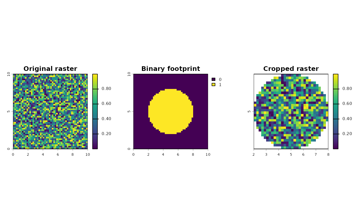
The function bin2crop() crops a continuous raster
according to a binary footprint (0/1).
#Continuous raster
r_cont <- rast(
ncol = 50, nrow = 50,
xmin = 0, xmax = 10,
ymin = 0, ymax = 10)
values(r_cont) <- runif(ncell(r_cont), 0, 1)
names(r_cont) <- "suitability"

#Binary footprint (circle around centre)
r_bin <- rast(r_cont)
xy <- terra::xyFromCell(r_bin, 1:ncell(r_bin))
dist_center <- sqrt((xy[, 1] - 5)^2 + (xy[, 2] - 5)^2)
values(r_bin) <- ifelse(dist_center <= 3, 1, 0)
names(r_bin) <- "footprint"

#Crop continuous raster to footprint
r_cropped <- bin2crop(r_bin = r_bin, r_cont = r_cont)

r_cropped
#> class       : SpatRaster
#> size        : 30, 30, 1  (nrow, ncol, nlyr)
#> resolution  : 0.2, 0.2  (x, y)
#> extent      : 2, 8, 2, 8  (xmin, xmax, ymin, ymax)
#> coord. ref. : lon/lat WGS 84 (CRS84) (OGC:CRS84)
#> source(s)   : memory
#> name        : suitability
#> min value   : 0.001161998
#> max value   : 0.999194679

par(mfrow = c(1, 3))
plot(r_cont, main = "Original raster")
plot(r_bin, main = "Binary footprint")
plot(r_cropped, main = "Cropped raster")